mod-EC
Datasheet
Procedure
Following good lab procedures is important to obtain the best results while also staying safe. Aside from safety considerations, the following is a step-by-step process calibration:
- Collect all the materials needed: calibration solutions, clean water, towels, equipment, etc.
- Rinse the probe in clean water. RO/DI, deionized, or distilled water is best. Tap off excess water drops trapped in the probe tip and blot dry. For lab probes, do not touch the electrodes inside the glass loop
- Pour some calibration solution into a separate container. It should be enough to fully submerge the tip of the probe, then submerge the probe.
- Continually take measurements, watching for the measurement to stabilize. Eventually, only the third decimal place will vary from measurement to measurement. When the reading stabilizes, have the module calibrate itself for the solution.
- Safely dispose of the calibration solution and clean or dispose of the container.
- Repeat steps 2 through 5 for each calibration point. When calibrating, use the labeled value, not the temperature-adjusted value.
Calibration Types
The module supports three methods of calibration.
Single Point
Single point is the least useful and should generally not be used. It uses one point and is only accurate for a small range around that one point.
Dual Point
Dual point calibration is used for measuring between two set points. To determine the points, decide on the lowest point to be measured and the highest point. After calibrating between those two points, the measurements can be expected to be very accurate between them. Outside the two points, the measurements will get increasingly inaccurate the further from the calibration points the measurement gets.
Triple Point
The module’s response is not perfectly linear throughout the entire range of possible measurements. To get the most accurate measurements over the widest range, triple point calibration can be used. It is similar to dual point, but uses three points rather than two. A good starting point for a very large range would be a low of 0.5 mS, a mid of 1.0 mS, and a high point of 10.0 mS.
Precedence
The module will select the best calibration type from the available calibrated points as follows:
- If there are high, mid, and low points, it will use triple-point calibration to calculate the result.
- If there are high and low points, it will use dual-point calibration to calculate the result.
- If there is a single-point calibration data, it will use single-point calibration to calculate the results.
- No calibration points used will result in an uncalibrated measurement.
Calibration data is stored on the module. Measurements will automatically use calibration data; there won’t be a change until both a high and low point have been entered.
More Explanation
The same solution can measure over a relatively wide range as the temperature changes. As an example, suppose a tank of water needs to maintain an EC value of 1.0 mS/cm. The tank is exposed to the weather, and the temperature increases and decreases throughout the day. The conductivity will also increase and decrease as the temperature changes. To have a reliable method of comparing the current conductivity to the setpoint, the temperature must be compensated for. This is done by choosing a particular temperature to adjust all readings to. This is typically 25 °C. The compensation would have the effect of changing the conductivity measurement taken at the current temperature and adjusting it so that it would represent what it would have been at 25 °C.
Several points of data are needed for this calculation:
- The solution’s current temperature
- The temperature to adjust to
- The temperature coefficient
The solution’s temperature and the temperature to adjust to have been discussed above. The temperature coefficient is the percent change per degree. The coefficient is different for every solution and is determined by its composition. Sometimes the solution being measured is known, and a temperature calibration characterization can be done, oftentimes the exact composition isn’t known, and an estimation is required. For freshwater, the most typical coefficient is 0.019. For seawater, it is around 0.021, and for pure water, 0.052.
Because the coefficients are estimations, they introduce a small amount of uncertainty. It is important to note that a chart of the measurement with varying temperature won’t be perfectly flat, indicating that all the temperature effects have been fully eliminated. It will still move with the temperature, but not nearly as much.
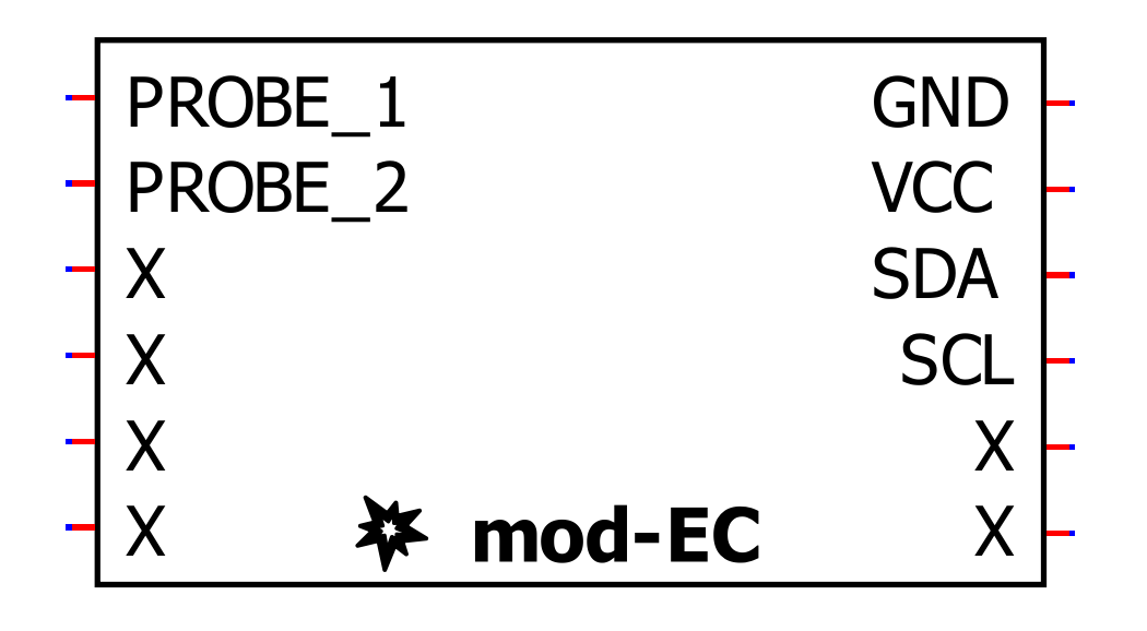
| Pin | Function |
|---|---|
| PROBE_1 | Provides a connection to the first electrode of an EC probe |
| PROBE_2 | Provides a connection to the second electrode of an EC probe |
| GND | Ground for the module |
| VIN | 3.3-volt power supply |
| SDA | Data line for I²C interface |
| SCL | Clock line for I²C interface |
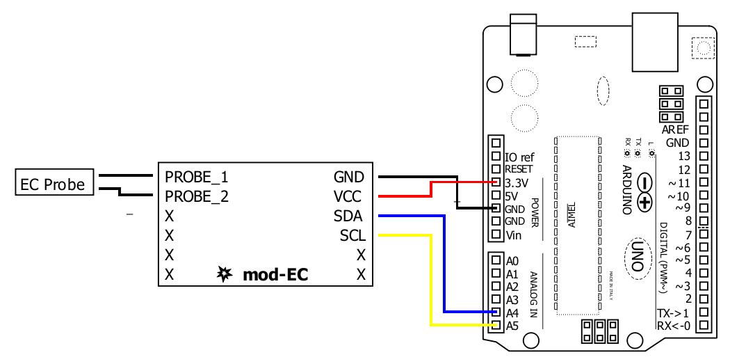
Wiring directly to a host controller
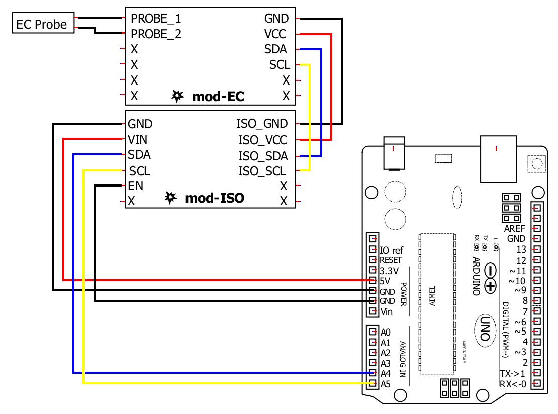
Using a mod-ISO module for isolation
1.
🔽 Install Arduino IDE
Install the Arduino IDE
2.
📦 Install the library
Start the Arduino IDE, press the Sketch menu, and then Include Library > Manage Libraries. Search for Microfire_Mod-EC and install the library.
3.
🔢 Code
Below is the Basic example. It can be found in File > Examples > Microfire_Mod-EC > Basic in the Arduino IDE.
4.
➡️ Upload the code
Pick the board and port, then Upload the code.
5.
🔎 View the output
Open the Serial Monitor, measurements should be displayed in the monitor, with updates every second.
6.
📒 Documentation
The library is documented here:
1.
📦 Install ESPHome
Follow the instructions on the ESPHome website.
2.
⌨️ Start a project
Type esphome wizard mod-ec.yaml in the terminal. Make sure the path on the terminal is where you want the project to be. Follow the steps, and there should be a .yaml file in the directory you ran the command in. For this write-up, it will be mod-ec.yaml. If you type esphome compile mod-ec.yaml you should see the project compile.
3.
🔢 Code
The YAML file should be changed to the following:
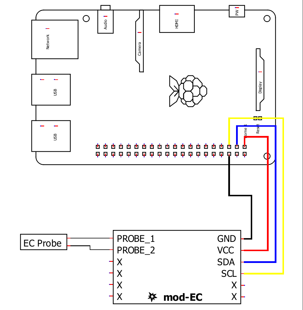
Wiring
1.
📦 Install the library
The Python library can installed through pip in a terminal:
pip3 install Microfire-Mod-EC
Typing python3 -m Microfire_Mod_EC.shell will start the shell application and give access to all features and functions of the module. Type help to see a listing of the commands available.
2.
🔢 Code
Create a python script and run the following sample code.
3.
📒 Documentation
The library is documented here:
This section documents the security properties of mod-EC. It is written for integrators who embed mod-EC in their own products, including manufacturers with obligations under the EU Cyber Resilience Act (CRA).
Classification
Mod-EC is a 3.3 V electrical conductivity sensor module with an I²C digital interface and on-module calibration processing. It is a “product with digital elements” in scope of the CRA. Its core function is measuring conductivity; the I²C interface is a local board-level data connection, not a network interface, and the module’s security functionality is not intended to secure other products or services. Mod-EC is therefore treated as a default-category product (not an Annex III “important product”), permitting self-assessment (Module A) without a notified body. The main CRA product requirements, CE marking, and technical documentation apply to units placed on the EU market from 11 December 2027.
Security Architecture
Mod-EC has:
- No network interfaces (no Wi-Fi, Ethernet, Bluetooth, or any wireless or cloud connectivity)
- No login system, user accounts, or credentials
- No storage of personal or customer data
- No host software that runs outside of your application; the supported libraries are open-source code that runs on your controller, not on the module
Persistent state on the module is limited to calibration constants, which are written by explicit calibration commands and retained across power cycles.
Trust Model
The I²C bus is assumed to be a trusted, local bus under the physical control of the integrator. The module performs no authentication, authorization, or encryption on I²C. Any device with electrical access to the bus can:
- Read measurements
- Issue calibration commands, which modify the calibration constants stored on the module
- Reset calibration to the factory state
Consequences: an attacker with bus access (which generally requires physical access to the host system) could corrupt calibration data or recalibrate the module, causing inaccurate EC readings. The module has no mechanism by which a remote party can reach it; exposure is entirely a function of the host system’s design.
Integration Guidance
If your finished product has CRA obligations, you may rely on this documentation and our CE Declaration of Conformity (available on request for units placed on the market after 11 December 2027) as part of your component due diligence. We recommend you also:
- Treat the I²C bus as a privileged interface; do not expose it to untrusted peripherals or externally reachable interfaces
- Apply plausibility checks and range limits to EC readings before using them for dosing, control, or other automated decisions, so that a corrupted reading cannot cause unsafe action
- Consider the mod-ISO isolation module for galvanic isolation where wiring runs outside your enclosure
- Remember that mod-EC is an environmental monitoring device and is not sold for medical or critical-use applications, per our terms
Version Identification, Reset, and Remediation
- The firmware version of a module can be identified through the supported libraries; the datasheet (link at the top of this page) documents the exact method. Library versions are published in the Arduino Library Manager and on GitHub.
- Calibration can be returned to the factory state with an explicit calibration reset command; there are no other user-configurable settings.
- Mod-EC does not update its own firmware over I²C. If a firmware vulnerability is confirmed, Microfire will provide mitigation guidance to integrators and remediation by reflash instructions, a reflash service, or replacement of affected modules.
Support Period and Reporting
Mod-EC versions receive security support for at least five years from the date they are placed on the market. To report a security vulnerability in mod-EC, its firmware, or our libraries, see our security page or email security@microfire.co.